Overview of Physical Proof

<Visual and Mathematical Demonstration>

Overview of Applications

Excel Spreadsheet using <HITRAN spectral data for CO2>

<Excel Method Explained>

<Earth Temperature by Excel>

Each column of the Excel spreadsheet has a programmed function that is automatically executed

if any change is made elsehwere in the spreadsheet. These are described in the manuscript and Supporting Information.

The common changes are to introduce a new spectral data file in columns A and B or a new CO₂ ppm value in column D.

Igor Spreadsheet Applications using <HITRAN data> for Visualization

<Igor Method Explained>

<Earth Temperature by Igor>

Igor functions are available to implement the calculation of new values of transmittance

and temperature.

<Calculate_Temperature()>

<Calculate_Tau()>

<Calculate_Transmittance()>

These macros (functions) are already available in the Earth_Temperature.pxp Igor file.

Each function accepts the CO₂ partial pressure as an input. For example,

Calculate_Temperature(0.00042) on the command line executes all columns of the spreadsheet

including all graphs appropriate to atmospheric concentration of 420 ppm CO₂.

The tools on this page using Excel, Igor Pro, and Python permit an observer to see the demonstration step by step.

QED: Calculation of Temperature vs CO₂ ppm

Obtaining HITRAN data

<HITRAN Website>

In the example we have used, we select CO₂ gas, na for natural abundance between 200 cm^-1 and 2400 cm^-1

This corresonds to 67091 transitions, which are not evenly spaced. The fortran program hgc.f [HITRAN Gaussian conversion]

creates a spectral data file of even spaced points with a separation of 0.01 cm^-1

The program requests an input file in comma separated files, which is the default output from HITRAN.

This corresonds to 67091 transitions, which are not even spaced. The fortran program hgc.f [HITRAN Gaussian conversion]

creates a spectral data file of even spaced points with a separation of 0.01 cm^-1

The program requests an input file in comma separated files, which is the default output from HITRAN.

Program requires input of the Doppler linewidth, which we have taken to be 0.13 cm^-1.

<Download HITRAN Gaussian conversion code>

The code can be compiled using the command line $ gfortran hgc.f -o hgc

The input HITRAN file is <CO2_na_hitran.csv>

The user may include isotopologues or even a superposition of methane and CO₂

Ozone, nitrous oxide, and other gases can also be included as desired. These are simply

added to the list of HITRAN transitions provided as input to the hgc fortran program.

H₂O could be added, but water enters the problem as a feedback that fluctuates rapidly.

For this reason we have followed other researchers who treat water as a global average.

The output file from this program can be used to replace the first two columns of either the Excel

or Igor spreadsheets, which will automatically calculate absorbance, transmittance,

the Planck function at 288 K and the product of Planck function and transmittance.

The integral of these last two quantities is used to calculate the global transmittance.

Column A consists wavenumber values (cm^-1).

There are 240,000 wavenumber values from 0.01 to 2,400 used as the independent variable for all other columns.

Column B (plotted vs A) is the CO₂ bending mode spectrum based on HITRAN.

This output is plotted in:

<Excel: Spectrum of CO2 (wait for Excel to downloand and open)>

<IgorPro Pdf: Spectrum of CO2 converted to pdf>

Column C

The constants P_atm/M_CO2g at 1 atm of pressure are multiplied by CO₂ mole fraction in columnd D.

Column D

The mole fraction of x_CO2. Enter a new value here to calculate new transmittance.

The transmittance multiplied by the Planck emission is used to calculate the Earth's surface temperature.

Column E

This column is the cross-section number density in one square meter above the Earth's surface.

This is the product of the previous two columns C and D, u_TOA=P_atm/M_CO2g.

Column F

F is the effective absorbance of CO₂ per square meter.

F (= B * C * D) or F = B * E.

Column G

G is the simple transmittance G = 10^-F. It is the fraction of radiation that passes through the atmosphere at a given wavenumber.

Column H

H is a correction to the transmittance based on numerical integration.

It converts the spectral point source into a radiation flux per square meter.

H = (10^-1.245F + 10^-0.13F)/2

Column I

I is the corrected transmittance converted from absorbance in column B and the cross-sectional number density in E.

It also converts the spectral point source into a flux.

I = (10^-2.245BE + 10^-1.13BE)/2

The output is plotted in column I of the Excel spreadsheet:

< CO2_Transmittance>

<IgorPro Pdf: Transmittance of CO2 converted to pdf>

Column J

J is the temperature in the calculated Planck distribution. The default used is 288 K.

Column K

K is the Planck distribution at temperature J. Visualize it in a plot of column K.

<Planck_Distribution>

Column L

Column L is the Planck distribution times the transmittance in column I.

Both K and L are plotted for comparison in

<Planck_Distribution and CO2 Transmittance>

<IgorPro Pdf: Integrated Transmittance of CO2 converted to pdf>

Visualizing integration

We can visualize the steps of integration of the Planck distribution with and without CO₂ transmission.

The global transmittance, tau_atm is the ratio of the integral (shown here as the sum) at each value of CO₂ to I₀ the intensity of radiation emitted by the bare earth.

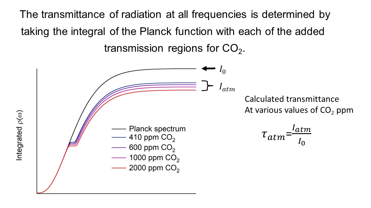
Each of these curves is the summation of Planck radiation with no CO₂ or varying ppm.

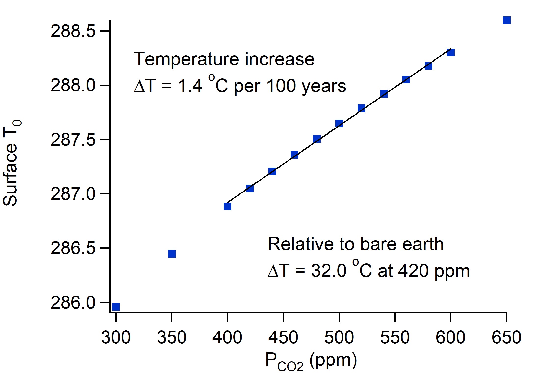
Column M Temperature and Transmittance vs. CO₂ ppm

The M column contains a global average transmittance of CO₂ and the temperature at the Earth's surface.

By calculating a number of different temperatures, transmittances, and CO₂ ppm

we can visualize the temperature effect at the Earth's surface as CO₂ increases.

Python code for visualization

Each of the python scripts is a standalone application.. They carry out all the operations of the Excel spreadsheet.

Converting HITRAN data to a Gaussian or Lorentzian broaded extensive spectrum.

Column B: The HITRAN spectrum of CO₂ calculated using line broadening.

Column I: The transmittance of CO₂

Columns K and L: Planck distribution (K) and product with The transmittance of CO₂ (L)

Integrated Planck curve and Planck times CO₂ curve.

The transmission and temperature as a function of CO₂ ppm are given by:

The script will read the ppm values in co2_ppm_full.txt and use the transmittance at a given value of CO₂ ppm to calculate the temperature.

Single point calculation of temperature as a function of CO₂ ppm is given in:

Caveat: the Python code can process at least 24,000 data points. The result obtained is qualitatively similar, but slightly smaller. This is due to a resolution effect since the Python integration has steps of 0.1 cm^-1, while Excell can handle 0.01 cm^-1. We welcome any improvements.

Data input files

• <co2_ppm_full.csv>: column of ppm values from 300 to 1000 → needed for <plot_co2_ppm_vs_temp.py>

• <co2_ppm.csv>: two ppm values 410 and 1000 needed for <planck_transmittance_compare.py> and <planck_transmittance_int_compare.py>

• <co2_bending.csv>: HITRAN data for CO₂ bending needed for all scripts
• <co2_bending_stretch.csv>: HITRAN data for CO₂ bending and stretching needed for all scripts using the complete set of vibrationsl for CO₂

• <hitran.csv>: HITRAN data for CO₂ bending and stretching used in hitran_to_gaussian to convert to the peaks with a Gaussian width of 0.13 cm\^-1\ with a spacting of the wavenumber of only 0.01 cm^-1. This file contains the 67,000 lines of CO^{2 bending and stretching vibrations. The python script rewrites those peaks preserving their intensity but broadening them and plotting them on a uniform spectroscopy base of 0.01 cm-1 in Excel. At present the python scripts run at 0.1-1, which means that only 24,000 data points are used to integration. This apparently reduces the accuracy of the result, but the ease of use suggests that python may be developed to help design the educational message.}