The Franck-Condon Factor
If we picture the vertical transition from ground to excited electronic state as occuring from a vibrational wave function that gives a probability distribution of finding the nuclei in a give region of space we can determine the probability of a given vibrational level from the overlap integral Sv’,v which gives the overlap of the vibrational wave function in the ground and excited state. The v’ quantum numbers refer to the ground state and the v quantum numbers refer to the excited state. As discussed in the lecture notes the total transition probability is the square of the transition moment. The transition moment can be separated into electronic and nuclear parts using the Condon approximation.
Condon approximation
: the electronic transition occurs on a time scale short compared to nuclear motion so that the transition probability can be calculated at a fixed nuclear position.
Note that this is a more restrictive approximation than the Born-Oppenheimer approximation. The B-O approximation states that nuclear and electronic motions can be separated, but does not demand that the nuclear coordinate be a fixed value.
Recall that the transition probability or transition rate in an electromagnetic field is proportional to the square of the transition moment. Given the Condon approximation we can write the transition probability as a product of an electronic term and a nuclear term.
B
µ |mge|2FCWhere FC refers to the Franck-Condon factor which is the nuclear term. The FC factor can be expressed as the square of nuclear overlap terms.
Note that we must sum over all vibrational states of the ground and excited state in order to calculate the Franck-Condon factor. In reality this sum is limited by the fact that only a finite number of states have significant overlap and can contribute to the absorption line shape. In this tutorial on the Franck-Condon factor we will
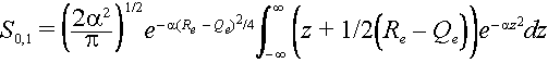
The nuclear overlap for the zero-zero transition S0,0 can be calculated quite simply using the definition of the Gaussian form of the wave functions.
![]()
Ground State Excited State
The nuclear overlap integral is

The exponent can be expanded as
and we use (Re + Qe)2 = Re2 + Qe2 + 2ReQe and (Re - Qe)2 = Re2 + Qe2 - 2ReQe to substitute and complete the square inside the integral. We can express Re2 + Qe2 = ½[(Re + Qe)2 + (Re - Qe)2].
Thus integral is
The integral is a Gaussian integral. You can show that if we let z =
Öa{R-1/2(Re + Qe)} then dz = ÖadR and the integral becomes.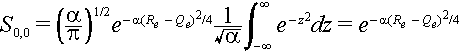
We could continue and calculate that overlap of the zeroth level in the ground state with all of the vibrational levels of the excited state S0,1, S0,2, S0,3, etc. Note that the Franck-Condon factor is the square of each of these terms S0,02, S0,12 etc. Each term corresponds to a transition with a different energy since the vibrational levels have different energies. The absorption band then has the appearance of a progression (a Franck-Condon progression) of transitions between different levels each with its own probability.
To calculate the overlap of zeroth ground state level with the first excited state level we use the Hermite polynomial H1(x) =2x for the excited state. Here x =
Öa(R - Qe)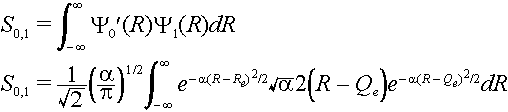
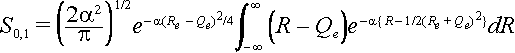
The same substitutions can be made as above so that the integral can be written as
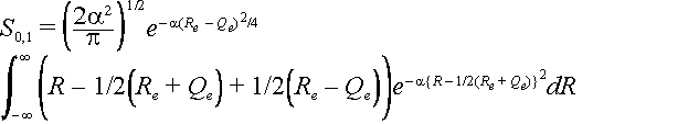
Let z = R – ½(Re +Qe) then the integral becomes
The integral can be broken into two parts.
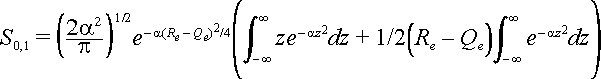
The first integral is zero and so the result is
![]()
We notice that the nuclear coordinate shift Re – Qe between the ground and excited states is a fundamental quantity. When multiplied by
Öa this position shift is given in units of the root-mean-square zero point displacement of the harmonic oscillator. We call this quantity D where D = Öa(Re – Qe). In these units the above expressions for the nuclear overlap factors become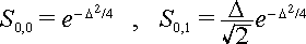
The energy associated with a displacement by
D is called S = D2/2, the electron–phonon coupling constant (also called the Huang-Rhys parameter). In units of S the overlap factors become![]()
The square of these terms are the contributions to the Franck-Condon factor. These are
![]()
We see that if only the zero level of the ground state is occupied that there is a fairly simple set of overlap factors that can be calculated. In the limit that
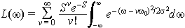
áw >> kT the entire progression can be calculated using
 .
.
In the above expression d is the delta function. The d-function states that there will be a line at an energy equal to váw and the spectrum will be zero elsewhere (see below for pictures and see the tutorial on lineshape functions for more information on the delta function). Notice that the above expression gives the Franck-Condon factor which is the sum of the squares of the terms S0,0, S0,1 etc. Also note the unfortunate confusing notation that S in the above expression. The terms S0,0 etc. are nuclear overlap factors and the term S is the coupling parameter between electronic excitation and nuclear coordinate displacements.
The displacement of the excited state potential energy surface is called D and it is given in units of the root-mean-square zero point displacement. The root-mean-square zero point motion is the average displacement of the nuclei in their zero point level. This can be obtained using
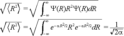
where

Note the extra factor of two in the definition of the zero-point displacement when compared to the definition of
D. Since D = Öa(Re – Qe) it might be more proper to say that the Öa scaling is proportional to the motion relative to the classical turning point since that is exactly Öa (see tutorial on r.m.s. displacement). The point is that D is dimensionless and gives a displacement relative to zero-point motion that can be compared in different systems. Therefore, both D and S can be used to describe spectra of different molecules.To understand the significance of the above formula for the FC factor, let us examine a ground and excited state potential energy surface at T = 0 Kelvin. Shown below are two states separated by 8000 cm-1 in energy. This is energy separation between the bottoms of their potential wells, but also between the respective zero-point energy levels. Let us assume that the wavenumber of the vibrational mode is 1000 cm-1 and that the bond length is increased due to the fact that an electron is removed from a bonding orbital and placed in an anti-bonding orbital upon electronic excitation.
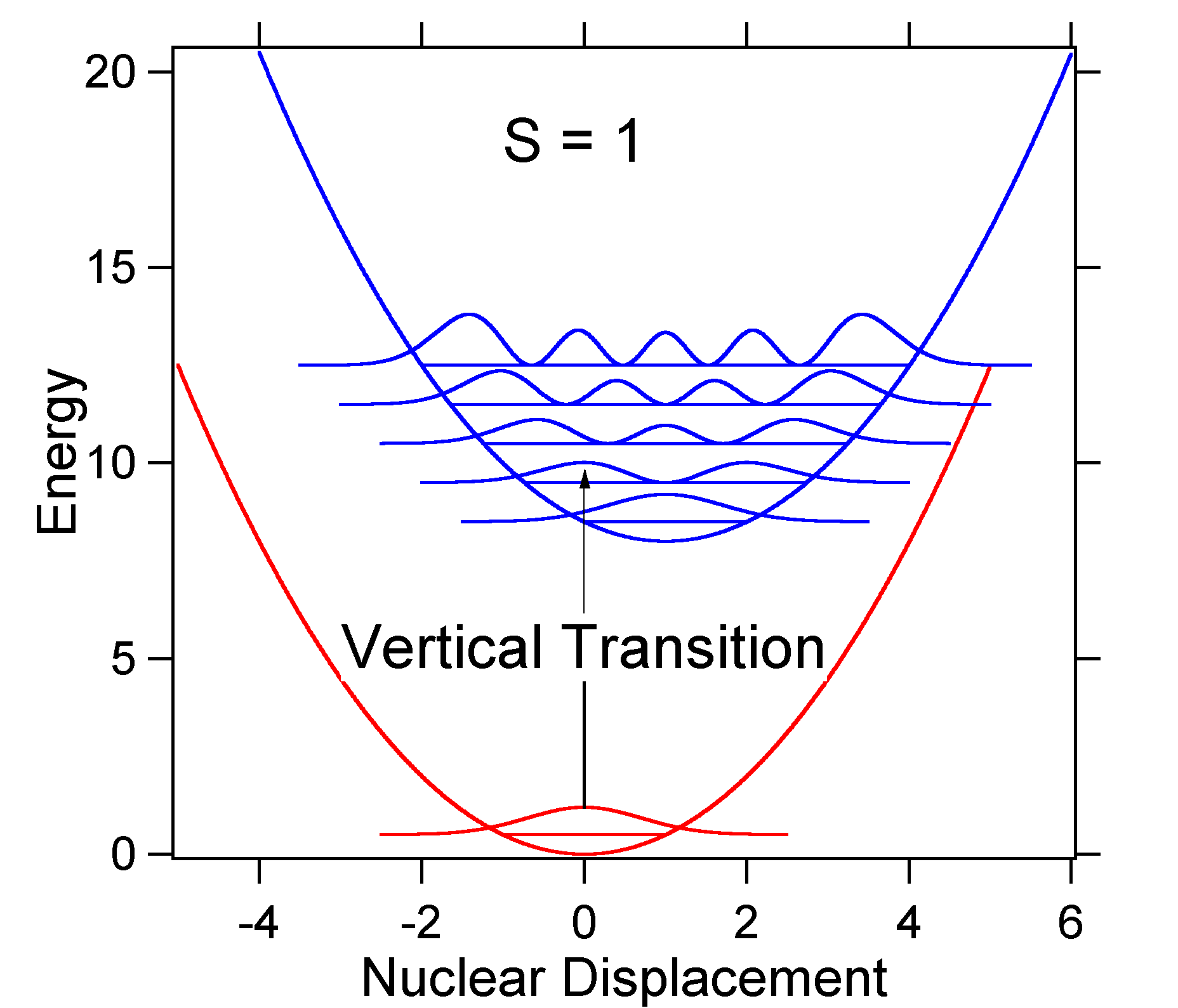
According to the above model for the FC factor we would generate a "stick" spectrum where each vibrational transition is infinitely narrow and transition can only occur when
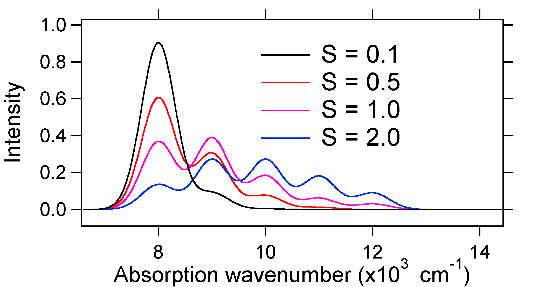
e = náw exactly. For example, the potential energy surfaces were given for S = 1 which implies that D = Ö2. The transition probability at each level is given by the sticks (black) in the figure below.
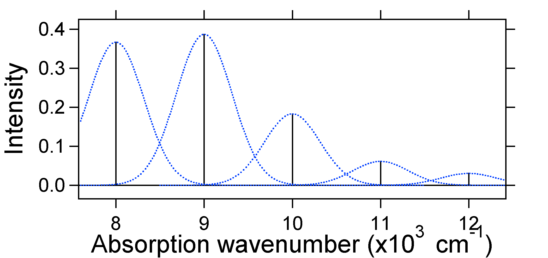
The dotted Gaussians that surround each stick give a more realistic picture of what the absorption spectrum should look like. In this first place each energy level (stick) will be given some width by the fact that the state has a finite lifetime. Such broadening is called homogeneous broadening since it affects all of the molecules in the ensemble in a similar fashion. There is also broadening due to small differences in the environment of each molecule. This type of broadening is called inhomogeneous broadening. Regardless of origin the model above was created using a Gaussian broadening
With
s = 1000 cm-1 i.e. a standard deviation of the order of the spectral line spacing. This is, of course, completely arbitrary and there are many condensed phase molecules where the broadening is greater than the line spacing leading to a completely smooth broad spectrum.The nuclear displacement between the ground and excited state determines the shape of the absorption spectrum. Let us examine both a smaller and a large excited state displacement. If
D = 1, then S = ½ and the potential energy surfaces in this case are: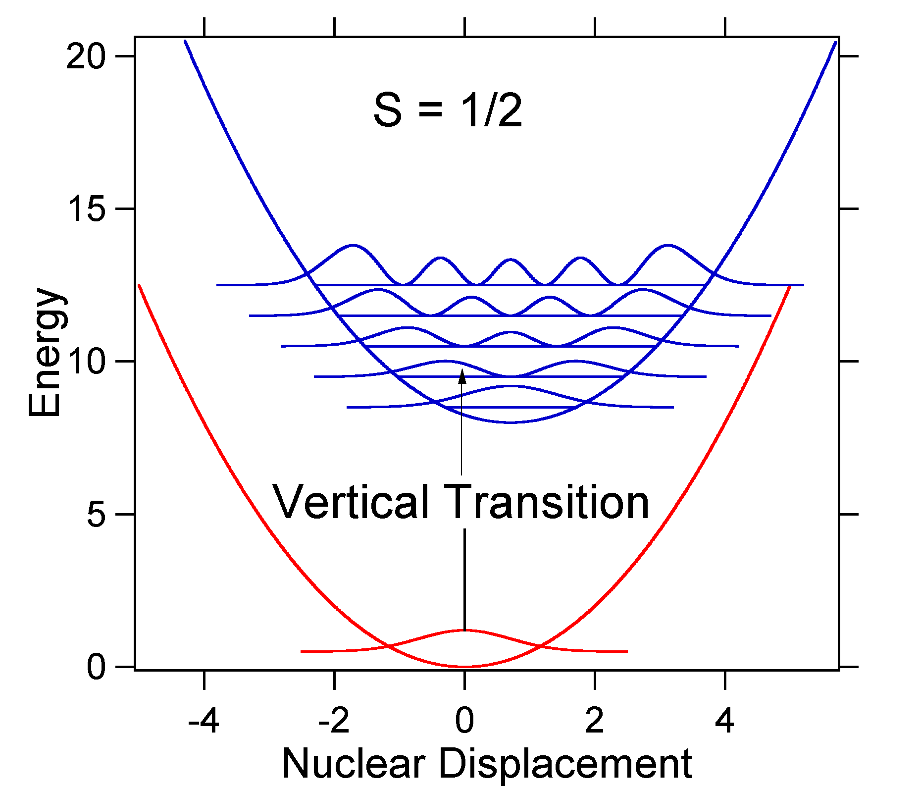
For this case the "stick" spectrum has the appearance

Note that the zero-zero or S0,0 vibrational transition is much large in the case where the displacement is small. As a general rule of thumb the electron-phonon coupling constant S gives the ratio of the intensity of the v = 2 transition to the v = 1 transition. In this case since S = 0.5 the v=2 transition is 0.5 the intensity of v=1 transition.
As an example of a larger displacement the disposition of the potential energy surfaces for S = 2 is shown below.
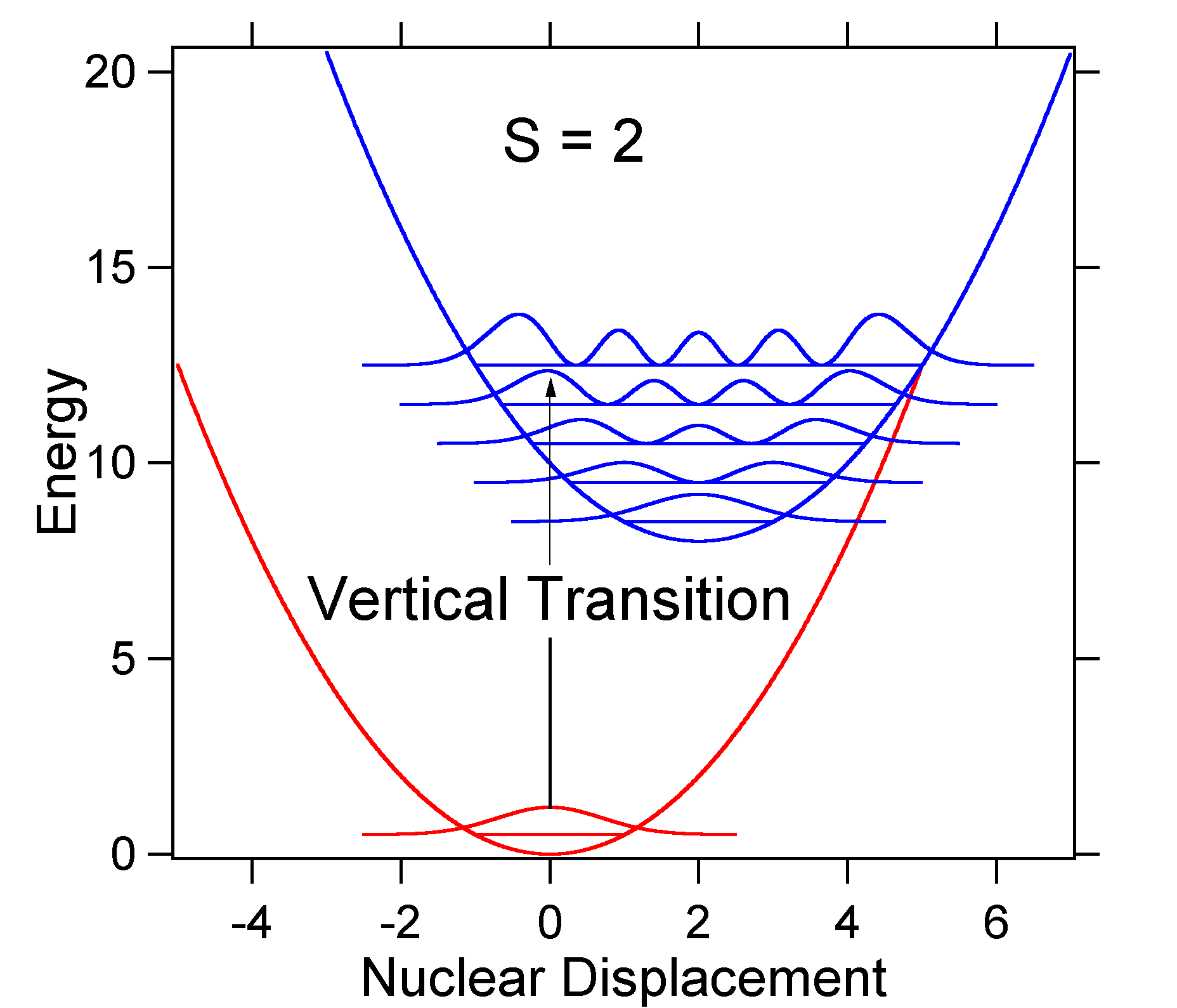
The larger displacement results in decreased overlap of the ground state level with the v = 0 level of the excited state. The maximum intensity will be achieved in higher vibrational levels as shown in the stick spectrum.

The absorption spectra plotted below all have the same integrated intensity, however their shapes are altered because of the differing extent of displacement of the excited state potential energy surface.